At Datacratic, working with data often means data visualization (or dataviz): making pretty pictures with data. This is usually more like making fully machine-generated images than carefully laying out "infographics" of the Information Is Beautiful school but I find they usually end up looking pretty good. There are lots of good tools for graphing data, like matplotlib or R or just plain old Excel-clone spreadsheets but what we use most often is Protovis, the Javascript library for generating SVG, coupled with CoffeeScript, which is a concise and expressive language that compiles down to Javascript.

The appeal of this combination for me is that it's a very data-centric, declarative way of writing code to generate graphics. If you read the code for some of the very pretty examples on the Protovis site, you'll see that they basically all have the same structure: a JSON-friendly object (usually an array) with all of the data to be visualized, and some small amount of code that declares how each element in that data object should be drawn. To me, the relationship between data and Protovis code is very similar to the relationship between semantic HTML and CSS: a separation of content and presentation. When we first started using Protovis to make pretty pictures, we'd do something similar to the Protovis examples: make an HTML file which contained a bit of markup and a script block with the Javascript code to call Protovis, plus a script tag in the header, which would load an external file which contained our JSON data, preceded by something like "this.data=". This suited us just fine, because the data to be visualized was usually the output of some Python or NodeJS or C++ process, and writing JSON to disk is really easy from pretty much any language.

The thing is, once you've written a bunch of similar dataviz code a few times, you look for a way to reduce the repetitive work, and so you pull your code out into an external file and you end up creating a whole bunch of very small HTML files to combine code and data. Say you've settled on a nice way of graphing a certain type of data, for example the output of a per-partition Click-Through-Rate vs Cost-Per-Click analysis script. You'll probably want to view the same graph for various partitions: per site, per vertical, per day of week, per time of day, whatever. So you generate a data file per partition, and you use the same code file, applied to each data file to generate each graph. And automating this task is just what the dataviz system that François and I built does.

At its core, it's just a very small PHP file which generates an page with script tags that include a data file on the one hand and a code file on the other, based on GET parameters. This allowed us to create a few reusable Javascript or CoffeeScript files which specified how to visualize certain types of data, and use this script to quickly pull up a page for a given combination of data and code to have the browser show us the resulting SVG. Of course we don't want to type GET parameters into the URL bar, so we wrapped this up in a little web-app that draws a file-tree based on what's on disk and lets you click on the file you want and loads up our core PHP file in an iframe. No sweat. But then things get interesting.

Because Protovis is so data-centric and declarative, each code file implicitly requires a certain format in its data: some scripts work on arrays of arrays, others on dictionaries. We decided to create a simple convention for how we name our files on disk so our web-app would know which data files went with which code files. For example, a file in the 'data' directory called 'stats-daily.js' could be visualized with a code file in the 'viz' directory called 'stats.js'. And then at some point we decided that some data formats could be visualized in more than one way, so we extended the code-file naming scheme to enable mixing and matching, say, data files named 'stats-daily.js' or 'stats-hourly.js' with code files called 'bargraph-stats.js' or 'scattergraph-stats.js' (see campaign example below). Essentially for a given data-type X, we have a one-to-many relationship with data files X-F1.js, X-F2.php etc and a one to many relationship with code files C1-X.js, C2-X.coffee etc. You'll notice from the file extensions in the examples just given that the data files don't have to be static on disk, they can be dynamically-generated with PHP. The code files can also be written in either Javascript or, my favoured option, CoffeeScript.

The next thing we noticed after having used this system for a while is that sometimes you want to compare or otherwise look at 2 datasets of the same format, side by side. So we added generalized support for "multi" visualizations, where you can check off which data files you want to pass to the multi-data-set visualization code.

So now whenever someone at the office wants to visualize some data, it's just a matter of having whatever code is generating this data output a JSON file to our 'data' directory with the appropriate name for the format, and our app will display links to visualize the file with whatever appropriate code files exist. And if the desired visualization doesn't exist yet, it's just a matter of creating an appropriately-named file in the 'viz' directory, which can then be reused to look at other data files in the same format. This makes for some nice collaborative workflows where we're all working on trying to build models that do the same thing and we can compare results really easily (see classifier example below).

Code & Demo

The code for our app is available on GitHub at https://github.com/recoset/visualize and a demo install of this code is available at http://visualize.recoset.com/ where you can see some sample data-sets and play with the UI. Google Chrome is the recommended browser for these visualizations as they're pretty memory and CPU intensive so Firefox has trouble with them, and they're SVG-based so IE has some trouble with that!

Classifier Example

If you go look at our demo, in the 'classifier' folder, you'll see 3 data sets. Each data set is the result of training and testing a different type of classifier to predict a certain type of conversion. The data set is an array of objects, each of which contains the results of running the classifier at a specific probability threshold. We can use this data to plot Receiver Operating Characteristic (ROC) curves, as well as Precision-Recall (PVR) curves and Lift curves. In the screenshot below, you can see the 'multi' option in action, plotting the results of our Boosted Bagged Decision Trees, Generalized Linear Model and Stacked Denoising Autoencoders against each other (they seem to perform about the same for this task).

Campaign Example

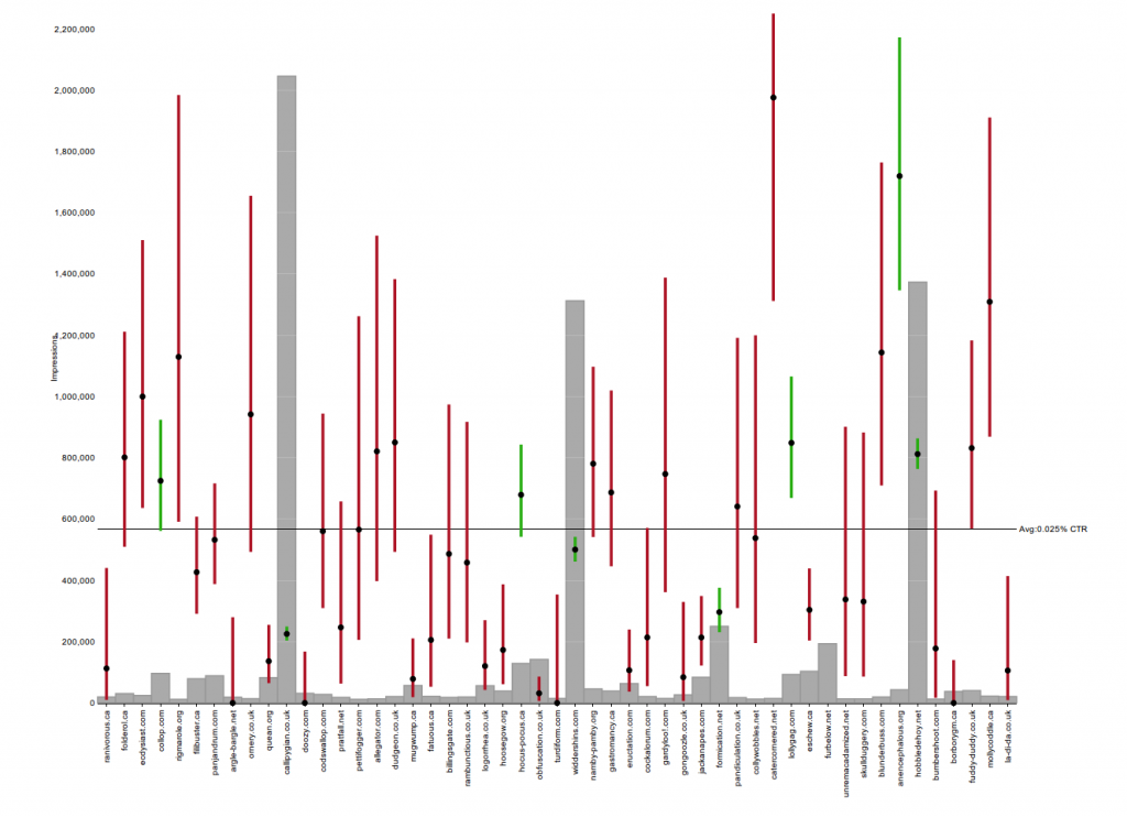
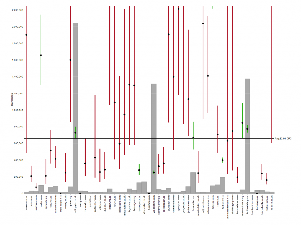
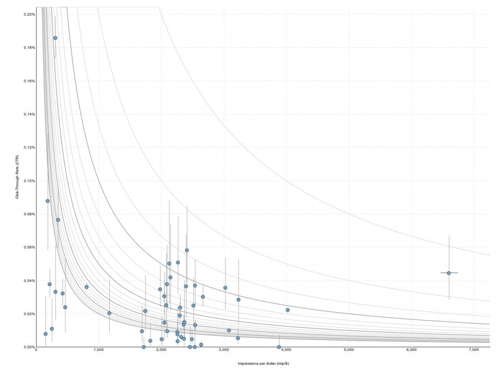
In the 'campaign' folder of our demo, you can see 2 datasets generated by our campaign-analysis system (note: this data has been obfuscated, and should not be interpreted as actual performance data!). The '50 top hosts' data is a good example of how we can visualize the same dataset in 4 different ways. In this case, the dataset is the performance of the 50 top hosts where we bought impressions over the course of this campaign. We can look at Click-Through Rate or Cost Per Click by host, (including confidence intervals!) or we can look at the relationship between these two quantities in a scatterplot. We can also look at a pie-chart of where we bought impressions. Same data, 4 views.

The second dataset in this folder allows us to draw what we call a campaign stream-graph. This is a visual representation of the progression of a campaign over time (day by day in this case, although we look at hourly versions as well). This graph shows various quantities of interest for each day of the campaign: impressions, total spend, CPC, CTR, CPM, site-mix etc. I encourage anyone interested in this visualization to go to our demo page and mouse over the various pieces of the graph.

One of the things we do at Datacratic is to use machine learning algorithms to optimize real-time bidding (RTB) policies for online display advertising. This means we train software models to predict, for example, the cost and the value of showing a given ad impression, and we then incorporate these prediction models into systems which make informed bidding decisions on behalf of our clients to show their ads to their potential customers.

The basic process of training a model is pretty simple: you  show it a bunch of examples of whatever you want it to predict and apply whatever algorithm you've elected to use to set some internal parameters such that it's likely to give you the right output for that example. A trained model is basically set of parameters for whatever algorithm you're using. Once you've trained your model, you test it: show it a bunch of new examples, to see if the training actually succeeded at making it any good at outputting whatever it is you wanted it to. The testing step often results in some datasets which we can feed into our data visualization system.

Now the bidding policies we've developed depend upon multiple such trained models, as mentioned above. Let's use the example of a policy P which depends on a value model V and a cost model C, so P(V,C). We won't need to train this policy per se, but we will want to run some simulations on it to test how good we would expect it to be at meeting our clients' advertising goals. We might come up with 2 different types of value models (say V1 and V2) and 2 different types of cost models (say C1 and C2) to train and test.  So we end up with 4 possible combinations of value and cost models and thus 4 different possible policies to test: P(V1, C1), P(V1, C2), P(V2, C1), P(V2, C2). Note that in practice, we will likely come up with many more than 2 variations on value and cost models, but I'll use 2 of each to keep this example manageable.

So how do we actually go about doing all this testing and training efficiently, both from the point of view of the computer and the computer's operator (e.g. me)? When you're just training and testing models independently of each other, you can easily get by with a simple loop in a script of some kind: for each model, call train and test functions. When you have some second step that depends on combinations of models, like the situation described above, you can just add a second loop after the first one: for each valid combination, call test function. This is how we first built our training and testing systems, but then we decided to parallelize the process to take advantage of our 16-core development machine.

While brainstorming how we might build something which could manage the sequence of parallel jobs that would need to run, we realized that we'd already been using such a system throughout the development of these models: make. More specifically: make with the -j option for 'number of jobs to run simultaneously'. The make command basically tries to ensure that whatever file you've asked it to make exists and is up to date, first by recursively ensuring that all the files your file depends on also exist and are up to date, and then by executing some command you give it to create your file.

Casting our training/testing problem in terms of commands which make can understand is fairly simple and gives rise to the diagram at the top of this page: rectangles represent files on disk and ovals represent the processes which create those files. The only change required to our existing code was that the train and test functions had to be broken out into separate executable commands which read and write to files.

 Here's the actual whiteboard brainstorm that led to this design 

Why not just parallelize our simple for-loops using some threading/multiprocessing primitives? Because using those kinds of primitives can be difficult and frustrating, while using make is comparatively easy and gives us a number of other benefits. Beyond the aforementioned -j option which gives us parallelism, the -k option makes it less painful for some steps to error out without having to build any specific error-handling logic: make just keeps going with whatever doesn't depend on the failed targets. And when we fix the code that crashed and re-make, make can just pick up with those failed targets, because all the rest of the files on disk don't need to be updated and essentially act as a reusable cache or checkpoint for our computation (unless they caused the crash, at which point you delete them and make rebuilds them and keeps going).

Having named targets also makes it easy to ask make to just give us a subset of the test results: it automatically runs only what it needs to to generate those targets we ask for. When you invoke make, you have to tell it what to make, in terms of targets, for example 'make all_test_results' or 'make trained_model_V1' etc. Adding new steps, such as the ability to test multiple types of policies, for example, or a 'deploy to production' step, becomes fairly trivial. Finally, the decomposition of our code into separate executables was actually helpful in decoupling modules and encouraging a more maintainable architecture. And whenever we get around to buying/building a cluster (or spinning up a bunch of Amazon instances), we can just prefix our executable commands with whatever command causes them to be run on a remote machine! So, armed with our diagram, and our excitement about the benefits that using make would bring us, we implemented a script which essentially steps through the following pseudo-code, given a single master configuration file that defines the models to be used:

1. for each command to be run (ovals in the diagram), generate a command-specific configuration file and write it to disk, unless an identical one is already there
   • Setup, training and testing configuration files for V and C models
   • Testing configuration files for P policies
2. for each target (rectangles in the diagram), write to the makefile the command to run and the targets it depends on, adding the configuration file to the list of dependencies
   • Setup targets for V and C models
   • Training and testing targets for each V and C models
   • Testing targets for policies P for each combination of V and C models
3. call make, passing through whatever command-line arguments were given (e.g. -j8 -k targetName)

Step 1 is helpful in allowing us to change a few values in the master configuration file, and having make only rebuild the parts of the dependency tree that are affected, given that make rebuilds a target only if any of its dependencies have more recent file modification dates. This means that, for example, I can choose to change some value in the master configuration file related to the training of C models, and when I call make again, it will not retrain/retest any V models. Doing this in effect adds dependencies from the various commands to certain parts of the master configuration file and lets make figure out what work actually needs to be done. And, let it be said again: it will do everything in parallel! Unfortunately, I don't have any code to put up on GitHub yet as the script we wrote and I described above is very specific to our model implementation, but I wrote this all up to share our experiences with this structure and how pleased we are with the final result!

I've written some follow-up posts to this one, as a series called Peeking into the Black Box, so I'm grandfathering this post in as "Part 0" of the series.

I read an interesting post on the AppNexus tech blog about their campaign monitoring tools and the screenshots there almost exclusively contained various pacing measurements. Some of the graphs there looked a lot like the ones I had sketched up while trying to solve the pacing problem for our real-time bidding (RTB) client. Here are the basics of the problem: if someone gives you a fixed amount of money to run a display advertising campaign over a specific time period, it's generally advisable to spend exactly that amount of money, spread out reasonably evenly over that time-period. Over-spending could mean you're on the hook for the difference, and under-spending doesn't look great if you want repeat business. And if you don't spend it evenly, you'll get some pissed-off customers, like this guy who had his $50 budget blown in minutes. Sounds obvious, right? Apparently it's harder than it looks!

Doin' it wrong

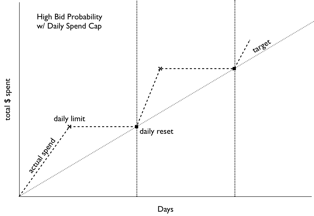
When Datacratic first dipped its toe into RTB (real-time bidding, characterized in this sister post), the main tool at our disposal to control budget/pacing was a daily spending cap. It took about 48 hours for us to figure out that that wasn't going to work for us: depending on the types of filters we used to decide when to bid at all, we'd either not manage spend the daily budget (more on that at the bottom) or blow the budget very quickly, usually the latter. In practice this meant that we would start buying impressions at midnight (all times in this post are in Montreal local time: EST or EDT) and generally hit our cap mid-morning.

On a daily spend graph over a 30-60 day period resulting from such a policy, this would probably look just fine: you're spending the budget in the time given, and spending exactly the right amount per day. But having this sort of 'dead time' where we don't bid at all bothered us, so as soon as we spun up our own bidder we added options like "bid on X% of the request stream" and when we looked at the resulting data we noticed something really interesting: the impressions we were buying before were actually among the most expensive of the day! The average win-price graph below (i.e. what the next-highest bid was to our winning one) from a high-bidding campaign shows a pretty clear pattern: if you start at noon, the dollar cost for a thousand impressions (the CPM) generally drops until precisely midnight, then jumps something like 40%. It fluctuates a bit, hits a high in the morning and then drops down again until noon to start the cycle again. This pattern repeats day after day:

So what's with that midnight jump? This is supposed to be an efficient marketplace, but are impressions a minute past midnight really worth 40% more than impressions 2 minutes earlier? Had we not had our initial experiences described above it might have taken us a long time to puzzle out! Our current working theory is in fact that there must be lots of bidders out there that behave just like our first one did: they have a fixed daily budget and they reset their counters at midnight. This would mean that starting at midnight, there's a whole lot more demand for impressions, and thanks to supply and demand, the price spikes way up (alternately, odds are that at least one of the many bidders coming back online is set up to bid higher than the highest-bidder in the smaller pool of 11:59PM bidders). And as bidders run out of budget throughout the day, at different times, depending on their budget and how quickly they spend it, the price drops to reduced demand. It's not obvious from the above graph but when you plot the averages over multiple days together there is a similar step at 3AM, when it's midnight on the West Coast, where a lot of other developers live and work and code:

Now there might be some other explanations for this price jump. We're in the Northeast and that impacts the composition of our bid-request stream, so maybe this is just a regional pattern (do other people see this also?) although the 3AM jump suggests otherwise. Midnight also happens to be when our bid-request volume starts its nightly dip, but that dip is gradual and isn't enough to alone explain that huge spike. Maybe some major sites have some sort of reserve price that kicks in at midnight. Or maybe everyone else is way smarter than us and noticed that click-through rates are much higher a minute past midnight than they are a minute before. I have trouble believing those explanations, though, so if anyone reading this has any thoughts on this I'd love to hear about them by email or in the comments below. Whatever the reason, it looks like if you're going to only be bidding for a few hours a day, don't choose the time-period starting at midnight and ending at 10AM!

Closed-Loop Control to the Rescue

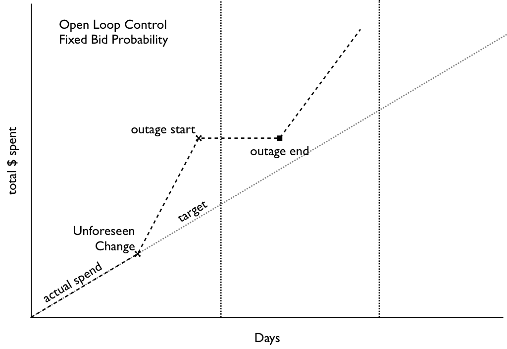
So let's assume that this post gets a ton of coverage among the right circles and that this before/after-midnight arbitrage opportunity eventually disappears, or maybe you just want to actually spread your spending evenly throughout the day, how would you do it? As I mentioned above, we have the ability to specify a percentage of the bid-volume to bid on. The obvious way to use this capability is to see how far into the day (percentage-wise) we get with our daily budget and bid only on that percentage of the bid-request stream, thereby ensuring that we run out of budget just as midnight rolls around. In practice, though, bidding on a fixed percentage of all requests can and does result in a different amount spent each day, sometimes higher than the daily budget (if you remove the daily cap) and sometimes lower. Maybe some days you get a different volume of bid-requests, because your upstream provider is making changes. Maybe there's an outage. Maybe the composition of your bid-request stream is changing such that all of a sudden the percentage of all bid-requests that's in the geo-area you're targeting goes way up (or down). Maybe your bidding logic doesn't result in a consistent spend. All of these factors could amount to a pretty jagged spend profile:

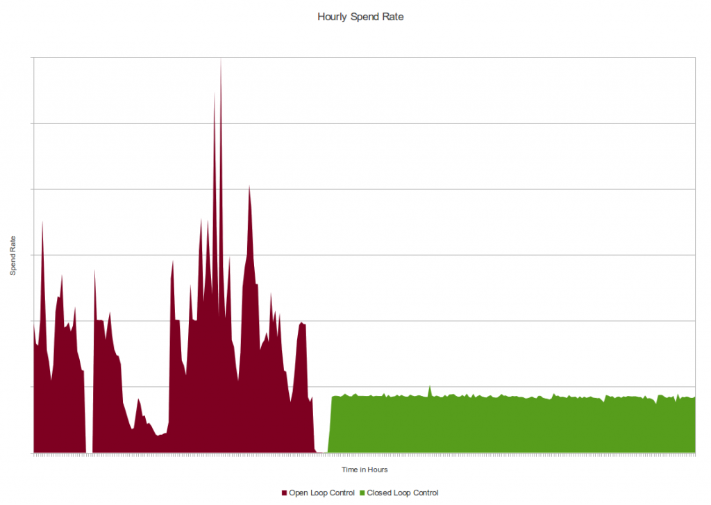
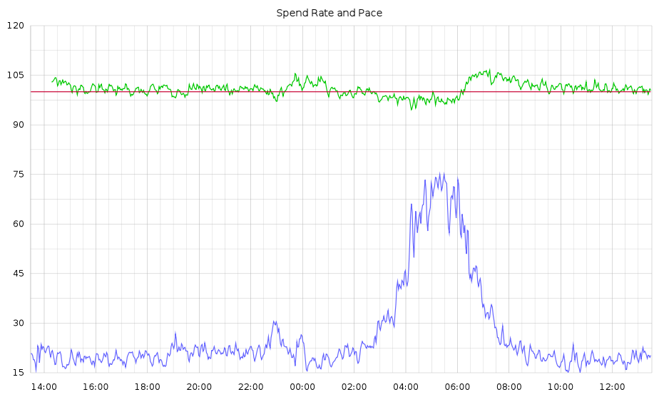
So what's the solution? For us it's to look at this problem as a control problem and to move from open-loop control to closed-loop control. If you theorize about the appropriate bid probability, set it up and let things run for a week and look at the results later, that's basically open-loop control. If every morning you look at what the spend was the day before and adjust the coming day's bid probability accordingly, you're doing a form of closed-loop control: you're feeding back information from the output into the input. It's pretty easy to automate (at least we thought so), and once that's done, there's basically no reason not to shorten the feedback loop from daily to every few minutes. Our RTB client was designed from the ground up to facilitate this sort of thing so we were able to control spend to within 1-2% of target with the following simple control loop: every 2 minutes, set the bid probability for the subsequent 2 minutes to that which would have resulted in the 'correct spend' over the preceding 2 minutes (maybe with a bit of damping). So if for whatever reason we get 20% fewer bid requests, for example at night, the bid probability will rise so that the spend rate stays roughly constant. There are more sophisticated ways to do closed-loop control, like the PID controller which I hacked into my espresso machine, but this really basic system works pretty well:

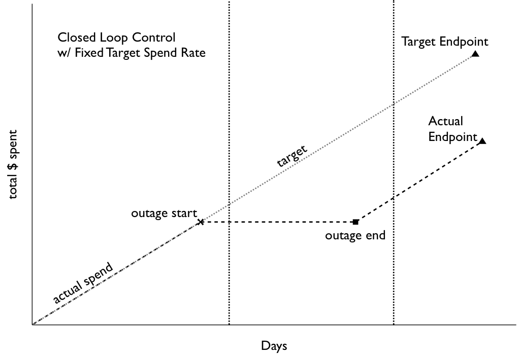
Like any good optimizer, the scheme described above does exactly what you ask it to: it tries to keep the error between 'instantaneous' spend rate and the target as close to zero as possible. If there's a full-on outage where no bidding occurs for an hour, this system will not try to make up the spend, it will just try to get the spend rate back to where it should be according to the originally-specified target, once bidding resumes:

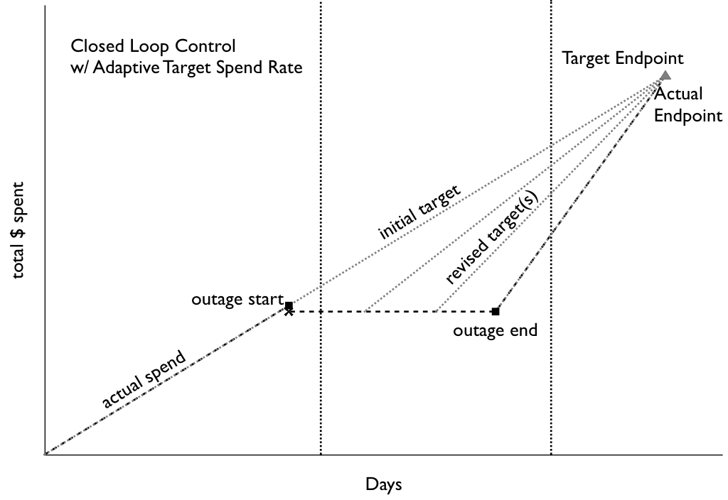
In order to deal with outages, as well as over- or under-spending due to accumulated error or drift from the instantaneous control system's imperfect responses, we have to dynamically adjust this spend-rate target as well. The way we've come up with to deal with this is to define the error function in terms of the original problem: continuously work to keep the spend rate at a level that will spend the remaining budget in the remaining time. This means that if there is an outage for an hour or a day, the spend rate for the rest of the campaign will be marginally higher to make up for it, without human intervention. This system also has the nice property of automatically stopping right on the dot when the remaining budget is zero:

Now obviously you might not want to always have exactly the same spend rate all the time, in fact I almost guarantee that you don't. A closed-loop control system can support pretty much whatever spending profile you like. You can also use one to manipulate other variables than the bid-probability (think: the actual bid price, or the targeting criteria, or whatever other scheme your quant brain can conjure up). Finally, the astute reader will notice that the approach described above is only really useful in situations where there is more supply than your budget permits you to buy, and so you need to allocate your budget over time. The approach above won't help at all if the optimal bid probability to meet your needs is up above 100%, that is to say that even when you bid on and win everything that matches your targeting criteria, you're not able to spend your budget. That's probably a topic for a different blog post.

Follow-up: I also posted this question on Quora, where I got a few responses. 

Follow-up posts: This post is now Part 0 of a series I'm calling Peeking into the Black Box. Check out Part 1 and Part 2 of the series, where I show how to really take advantage of other bidders' behaviour.

There doesn't appear to be a good Wikipedia entry for RTB for me to link at the moment, when I want to blog about it so I'll draft my own explanation here. (Edit: there is an entry now, but I like my characterization better!) Keep in mind while reading this that I'm looking at RTB as a software engineer with an interest in economics, rather than as an ad industry veteran!

What is RTB?

Real-Time Bidding (RTB) is a way for advertisers to pay publishers to show ad impressions on their websites. In this context, an 'advertiser' can be anyone with a product to sell: a car company, a small e-commerce website etc. A 'publisher' can be anyone with a website: a newspaper, a blogger, Facebook, Google etc. An 'impression' is a single instance of a banner ad being shown on a web page. The term RTB is usually not applied to other ad formats such as text ads ads, or ads alongside Google search results or Facebook news feeds, as different technology is used to buy and sell those other formats. The word 'bidding' comes from the fact that the price of impressions is set via an auction mechanism, where the role of the auctioneer is played by an 'ad exchange' who mediates between advertisers and publishers. The term 'real-time' stems from the fact that advertisers bidding in the auction must specify the price they are willing to pay for each impression separately for each impression, and within a strict time-constraint: usually around one tenth of a second, so the auction can run as the web page on which the impression will be shown is loading.

How does RTB work on Technical Level?

In terms of the technical aspects of participating in the auctions as a bidder, a computer subscribes to a stream of many thousands of bid-requests per second from the exchange, each one representing an impression to be shown very shortly. For each one, within the hard-real-time constraints, the computer must respond by specifying if/how much it wants to bid, in units of millionth of a dollar (u$). The cost of online advertising is usually discussed in terms of cost-per-mille (CPM) in dollars, so $1 CPM implies 1 million microdollars for 1 thousand impressions, or u$1000 per impression. The bidding computer can make its decisions based on the various attributes contained within the bid-request: the URL, the position of the ad spot in the page, the user's location and local time, the number of times this user has previously been shown a given ad, any additional data the bidder has on file or has purchased on that particular user, etc.

What do RTB Auctions Look Like?

From my reading on auction theory, here is how I would characterize what goes on in most RTB auctions:

• There exists a sequence of auctions to sell impressions, and the participants (bidders) are not always the same from auction to auction.
• The auctions are closed (aka sealed-bid) and single-round, so participants do not see each other's bids. All bidders submit their bids once and the winner is determined.
• The auctions are second-price, so the winner is the person who bids the highest, but pays whatever the amount of the next-highest bid was. Incidentally, only the winner knows what the winning bid was, and they learn what the next-highest price was, also, because that's what they paid.
• The auctions are single-unit, in that participants are bidding on single ad impressions at a time.
• The goods being auctioned are perishable: you use them immediately when you buy them and then they're gone. They have no resale value.
• The goods being auctioned are slightly different from auction to auction: the history of the user who will be seeing the eventual ad the winner will show matters to each bidder, as does for example the time of day etc.
• The valuations are uncertain, in that each bidder only has an estimate of how much it is worth to them to win this auction, and usually not even a very good estimate.
• The valuations are independent, in that the value of winning the auction to each bidder doesn't impact the value of winning the auction to any other bidder.
• The valuations are private, in that the value of winning the auction to each bidder is not known to the others.
• Not every publisher is willing to sell to every advertiser, and vice-versa, due to various brand, appropriateness and competitive concerns.
• Publishers will sometimes set a reserve price: a price below which they will not sell, so as not to enable advertisers to use RTB to undercut existing sales channels.

These characteristics make the RTB marketplace fairly different from, say, a stock exchange, where people buy and sell large pools of indistinguishable units of stock, whose value is intimately linked with the price at which it can later be resold, and in general no one cares who is buying or selling.

Why?

Participating in RTB auctions is fairly technically challenging, and good bidding strategies are not obvious, so there must be some perceived advantage over the alternative. In this case the alternative is a complicated web of relationships between publishers and advertisers, sometimes with 'ad networks' and other middlemen in between. The purpose of RTB is to set up a more efficient marketplace for advertising inventory. One where fine-grained control over bids allows advertisers to save money by purchasing a smaller quantity of better targetted ads, even if they pay more per impression. One where publishers are able to earn more from their web properties because they can more economically reach the advertisers who are willing to pay a high price per impression for the ads they do show. And one where the end-users who actually see the ads are happier because they see fewer cheap and irrelevant ads. Now obviously, for buyers to spend less and sellers to earn more something has to give, and that's where the word 'efficient' comes in. Right now there is a lot of opportunity cost and operations cost on both sides of the market and RTB is meant to reduce a lot of that. Whether or not any of the promise of RTB is actually materializing for any side of the market equation is still an open question, and it's a rapidly-evolving area of the online advertising industry.

More Reading & Listening

Mike on Ads is a good blog by the CTO of AppNexus, which is a big company in this space. Here are a bunch of his posts on RTB. I've also enjoyed a few episodes of the Trader Talk podcast on RTB.

This article is about the statistical and economic theory that underlies Datacratic’s real-time bidding strategies, as a follow-up to my previous article on how we apply control theory to pace our spending, which I’m grandfathering in as “Part 0” of this short series.

At Datacratic, we develop real-time bidding algorithms. In order to accomplish advertiser goals, our algorithms automatically take advantage of other bidders’ sub-optimal behaviour, as well as navigate around publisher price floors. These are bold claims, and we want our partners to understand how our technology works and be comfortable with it.  No “trust the Black Box” value proposition for us. In Part 1 of this series I’ll explain the basics of our algorithm, first how we determine how much to bid, and then how we determine when to bid. In Part 2 I’ll show how this approach responds in some real-world situations.

First, Tell the Truth

Let’s say, for sake of illustration, that you are Datacratic's bidder.  You’re configured for a 3-month direct-response campaign with a total budget of $100,000 and a target cost-per-click (CPC) of $1.00.  Like every other participant in real-time auctions, you subscribe to a stream of several thousand bid requests (also known as ad calls) per second, each representing an opportunity to immediately show an ad to a particular user on a particular site. You must respond to each bid-request which matches your targeting criteria with a bid, within a few dozen milliseconds. How do you decide what amount to bid? Most real-time auctions are what are known as Vickrey, or second-price, auctions.  The winner is the one who places the highest bid, but pays the amount of the second-highest bid. This type of auction was likely chosen by the designers of real-time exchange because the best strategy for bidders in such a situation is to “bid truthfully” (one of the well-known results of auction theory). This means that the bid you place should be equal to the amount that the good is worth to you.  In this case the “good” is the right to show an ad.  How much is that “worth”? The target CPC is $1.00, so it’s not a bad assumption that a click is worth at least that much to the advertiser.  Let’s say that the average click-through rate (CTR) is 0.05% for this campaign: one out of every two thousand impressions gets clicked on.  So if you win this auction, you have a 0.05% chance of getting something that is worth a dollar, and multiplying those together we can say that the expected value of winning this auction is 0.05 cents.  If you’re bidding truthfully (which auction theory says you should), that’s how much you should bid.  One equation you could use to come up with a bid is therefore:

bid = value = targetCPC * CTR

That’s a bit too simplistic, though, and doesn’t take advantage of the real-time nature of the exchange.  We’re a predictive analytics company, so as our bidder you have access to some fancy models.  These models predict, in real-time and on a bid-request by bid-request basis, the probability that this specific user will click on this specific ad in this specific context at this specific time. This means that you don’t have to use the campaign-wide average CTR when computing your bid, you can use the probability that our predictive model has generated for this request:

 bid = value = targetCPC * P(click)

So far so good, but not particularly groundbreaking: where is the secret sauce, other than in the probability-of-click prediction model which is beyond the scope of this article? That predictive model is certainly part of it, but there’s actually an additional wrinkle to the above equation: it only tells you what the bid should be if you actually decide to bid. And when deciding whether or not to bid, you shouldn’t just look at the value of winning the auction, but the cost as well.

To Bid or Not To Bid, or: Cost is not Value

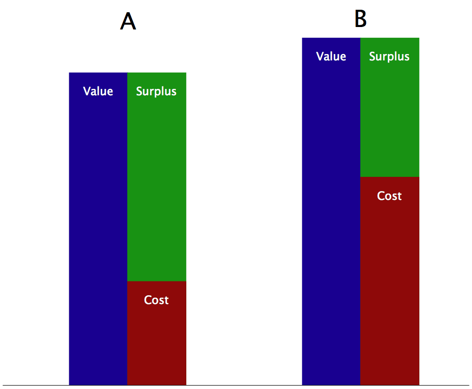
As I talked about in Part 0, if you just bid on every bid-request that comes your way, you’ll spend the budgeted $100,000 way ahead of the 3-month schedule. In that article I also detailed a system for spreading your spend out over time by using a closed-loop control system to vary the probability of a bid being submitted.  Let’s try to take that idea further: what if instead of randomly selecting which requests to bid on, you could find a way to bid on only the best requests? I just showed a way to model the expected value of winning an auction but in this context “best” doesn’t just mean “highest value”; that’s only half the picture. As an example of this, let’s look at an importer purchasing one of two types of goods for resale. Good A has a 10% lower resale value than Good B, but it costs half as much:

In this case the less valuable Good A is “better” because because what matters isn’t just the value or the cost but the difference between the two, or the surplus.  In business this is called profit and in game theory this is usually called the payoff.

surplus = profit = payoff = value - cost

The equation above holds for the RTB context if you win the auction, but what if you don’t? In that case, you get no chance at a click, so the value is zero, and you also don’t pay anything, so the cost is zero (modulo fixed costs, which are out of the scope of this article).  So for our purposes, the expected surplus is the same as above, multiplied by the probability of you actually winning the auction:

surplus = (value - cost) * P(win)

Now assuming that alongside Datacratic's click-probability predictor, you also have access to a clearing-price-predictor (again beyond the scope of the current article) that tells you for each bid-request how likely you are to win the auction at each price, you can now compute the expected surplus.  (As it happens, one can also maximize this equation as a function of the bid to prove the well-known “bid truthfully” result mentioned above: the bid which gives you the highest surplus, no matter the price distribution, is equal to the value).

So now when our closed-loop pacing control system says that in order to meet the budget requirements, you should only bid on a quarter of the request stream, you can choose to bid only on the bid-requests which have expected surpluses in the top quartile. This means that the control value is no longer the probability of bidding, but some measure of selectivity in the auctions you are willing to participate in: the lower the control value, the more selective you should be. You’re still placing the optimal bid every time, but now you’re specifically targeting the auctions where you think you will make the most profit given the target CPC, thereby increasing your chances of actually achieving a much lower CPC.

Algorithm Meets World

This post explains the two major components of our system: bidding truthfully and pacing economically. In Part 2 of this series, I’ll show how this approach to RTB handles some real-world situations advantageously.  

In Part 1 of this series, I claimed that Datacratic’s RTB algorithm is able to take advantage of other bidders’ sub-optimal behaviour and navigate around publisher price floor in order to achieve advertiser goals. I then described the algorithm, which applies what can be called a “bid truthfully, pace economically” approach. In this second part, I show how this algorithm can in fact live up to these claims.

When you bid truthfully and pace economically, you are always trying to allocate your budget to the auctions which look like the best deals, whether that means that the user is very likely to click, or that the price is low because fewer bidders are in the running or there is no publisher price floor.

How to Take Advantage of Other Bidders’ Behaviour

In Part 0 of this series, I showed that the average win-price for RTB auctions jumps up at midnight Eastern Time and described a pacing system which, if used by everyone, would prevent this jump, by spending at a constant rate. This system works by frequently updating a control value which is interpetted as the probability of bidding on any given auction. There is an implicit assumption underlying this system though: that any two randomly-selected bids are equivalent, regardless of, for example, the time of day. So while I introduced this system by talking about variability in the clearing price over the hours of the day, the simple pacer actually ignores this fact. This did not escape all readers of my post, some of whom commented in private that if we know the price is much higher at certain times, then we just shouldn’t bid at those times! Now that I’ve described the way we compute expected surplus on a bid by bid basis, I can explain a principled way for a pacer to simultaneously handle variability in clearing prices and impression quality that doesn’t involve hardcoding hours when not to bid. All that is needed is for the pacing system to update the control value much less frequently, say once a day, and to treat the control value as a “minimum acceptable expected surplus” threshold. Consider the following graph comparing the evolution of average clearing-price and average expected surplus over a few days, noting how at midnight the price jumps and the surplus drops:

A well-tuned, infrequently-updating pacing system will essentially draw a horizontal line across this graph, and our bidder will bid whenever the surplus is higher than this threshold. The key insight here is that the curves here represent the means of some fairly wide and skewed distributions. Even if the mean price goes up and therefore the expected surplus drops, that doesn’t mean there aren’t any “good deals” to be had: it just means there are fewer of them. By setting a hard, slowly-changing threshold, our bidder can continue bidding throughout the day, but it will probably spend less in the hour right after midnight than in the hour right before midnight. We like to say that this is taking advantage of other bidders’ sub-optimal behaviour because some bidders are irrationally piling into the market right after midnight and driving the price up. Our algorithm continues to “skim the cream”, bidding in the best-looking auctions, but does back off a bit, holding its budget in reserve for such times as other bidders have run out of money for the day. As that happens, the drop in demand causes a drop in clearing price and a concurrent rise in expected surplus, causing our bidder to spend more.

Navigating Around Publisher Price Floors

Having covered how our algorithm responds to the actions of other bidders, how about publishers? How does this system respond to publisher price floors? A price floor, or reserve price, is basically a statement by a publisher that they will not sell below a certain price. It’s almost as if a publisher is bidding on its own inventory. If there are no higher bids than the price floor, there is no transaction. If there is more than one bid above the price floor then the price floor does nothing and the winner pays the second price. If there is only one higher bid, however, that bidder wins and pays the reserve price. In this third case, the publisher gets some of the surplus from the auction that the winner would have gotten had there been no floor.

This all makes perfect sense at the micro level, as by definition if we win the auction, we were willing to pay more than we did: our bid was how much it was worth to us, and we paid the second price so the difference between the two is profit for us. Any publisher would rather that we had just paid them the entire bid amount so they could get that profit, and therefore they have an incentive to raise the price floor all the way to our bid amount to “capture back” as much of that surplus as they can. Our algorithm responds to a publisher price floor the same way it responds to the actions of other bidders causing the price to rise. At any given time, the pacer’s control value tells our bidder the minimum expected surplus required for it to bid. If a publisher raises their price floor (and if our price model captures this), the expected surplus of auctions for their impressions will drop. If it drops below the control value, we will simply not bid on those auctions at all, rather than accepting the higher price. This is what we call navigating around publisher price floors. The control value is set so that the budget will be met, and is based on the availability of surplus on the whole exchange, not just on any one publisher’s sites. In effect, this puts an upper bound on the price floor any publisher can set before losing our business, so long as we can get a higher expected surplus elsewhere. This upper bound will be lower than the value to us of winning the auction, but could still be higher than the next-highest bid, so we do give up some of the surplus to the publisher. This is pretty much the way the exchange should work: it’s a market mechanism which uses competition to divide up the surplus pie.

It’s worth mentioning that at the macro level, publishers don’t necessarily sell all their inventory on a spot basis on the RTB exchange: they try to sell inventory at a much higher price on a forward contract basis ahead of time. In industry jargon, inventory sold on a forward contract basis is called “premium” and everything else is called “remnant”. Without getting too deeply into this, publishers have an incentive to put up very high floor prices so that advertisers don’t stop buying expensive premium inventory because they think they can buy the same impressions more cheaply on the spot market (i.e. as remnant inventory). The industry lingo for this effect is “cross-channel conflict”, because the remnant "channel" is perceived to be hurting the premium "channel". If a publisher is using this type of rationale to set a price floor, they will likely set it higher than the amount of our bid, rather than trying to squeeze it in between the first and second highest bids. This would translate into an expected surplus of zero, as there would be no chance of us winning the auction. Again, our algorithm just doesn’t bid on this type of auction; it certainly doesn’t raise the bid value to win an unprofitable impression. Mike on Ads has a good post about why it’s a bad idea for publishers to do this, based on some hypothetical behaviour of bidders. Our algorithm can automatically implement the types of behaviour he describes.

Un projet sur lequel notre équipe d'apprentissage machine travaille actuellement est un engin de recommandation qui sert à générer des courriels personnalisés pour les clients d'un magasin en ligne. Le modèle que nous avons développé utilise l'historique de navigation et d'achats des utilisateurs du site. Chaque utilisateur est représenté par la combinaison de l'ensemble des produits avec lesquels il a interagi ainsi que leur relation avec chacun des produits que nous pouvons lui recommander.

Vers la fin du projet, un problème auquel nous avons fait face était de rendre possible l'exécution de notre modèle sur des centaines de milliers d'utilisateurs dans un temps très court. Nous aurions pu passer du temps à accélérer le modèle lui-même. Il y avait par contre un gain beaucoup plus grand à réaliser en changeant simplement la manière dont nous traitions chaque utilisateur.

Méthode séquentielle

À l'origine, chaque utilisateur était traité de manière séquentielle, c'est-à-dire que nous passions simplement à travers la liste des utilisateurs un après l'autre. En supposant une méthode score() prenant un identifiant d'utilisateur uid en paramètre et retournant la liste des scores pour l'utilisateur, chaque ligne de notre fichier de sortie a la forme suivante:

uid,s1,s2,s3,...,sN

L'algorithme séquentiel en Python ressemble à ceci:

with open("scores.csv", "w") as writer:
    for uid in uids:
        writer.write(score(uid)+"\n")

Après l'exécution, on se retrouvera donc avec un fichier scores.csv qui contiendra chaque utilisateur sur une ligne, suivi de tous ses scores associés.

Méthode MapReduce

Comment accélérer la génération des scores? Puisque les scores pour chaque utilisateur sont indépendants de ceux des autres, une manière simple est de générer les scores en parallèle selon le patron MapReduce et en utilisant de simples outils UNIX. La machine sur laquelle notre modèle est exécuté possédant 32 coeurs, nous pouvions tout exécuter en parallèle localement et potentiellement diviser le temps de calcul par 32 si chacun des coeurs générait les scores pour 1/32 des utilisateurs.

Rappelons que MapReduce est un patron qui comprend deux étapes: l'étape map consite à séparer un grand problème en n plus petits problèmes et de les traiter en parallèle, et l'étape reduce consiste à recombiner les résultats de l'étape map en un seul résultat.

Pour exécuter cette tâche en MapReduce, en plus du script générant les scores (appelons le score.py), nous aurons besoin d'un deuxième script qui aura comme tâche de démarrer plusieurs instances de score.py en leur disant quelle partie du travail effectuer.

Commençons par modifier score.py pour qu'il implémente la fonctionnalité map. Défnissons deux variables, total_nodes et node_num, respectivement le nombre total de noeuds de travail ainsi que le noeud actuel.

for i, uid in enumerate(uids):
    if Math.abs(i - node_num) % total_nodes != 0:
        continue
    print score(uid)

Nous avons fait deux petites modifications comparativement à la version séquentielle:

1. Au lieu d'écrire les scores dans un fichier, le script les retourne sur la sortie standard.
2. Une condition dans la boucle permet de sauter tous les utilisateurs pour lesquels nous ne sommes pas le noeud responsable.

Comme dit précédemment, le deuxième script est le contrôleur et est responsable de démarrer les noeuds de travail (étape map) ainsi que de combiner leur résultat (étape reduce). On peut exécuter le premier script en appelant simplement score.py et en passant en argument les variables total_nodes et node_num.

Pour exécuter les tâches en parallèle, nous utilisons GNU Parallel, dont nous avons déjà parlé dans un article précédent. Son utilisation se résume à spécifier une commande à exécuter où un argument sera substitué à partir d'une liste. Par exemple la commande suivante compressera en parallèle avec 12 coeurs tous les fichiers commençant par a_compresser.

parallel -j12 "gz {}" ::: a_compresser*

Pendant l'exécution de parallel, chacun des scripts score.pyécrira son propre fichier de résultats. Pour les combiner, nous n'avons qu'à exécuter cat sur l'ensemble des fichiers et de faire une redirection dans un autre fichier, ce qui combinera tous les fichiers dans un. Cette logique en bash ressemble à ceci:

C=32
parallel -j$C "score.py $C {} > scores-{}.csv" ::: `seq 0 $[C-1]`
cat scores-*.csv > scores-combined.csv

Adopter cette stratégie nous a donc permis de dramatiquement accélérer la génération des scores en utilisant pleinement les capacités de notre machine. La réduction en temps était linéaire puisque le goulot d'étranglement était le processeur. L'exécution parallèle prenait environ 40 minutes avec 32 coeurs, au lieu d'environ 21 heures de manière séquentielle. Cette accélération a pu être faite avec de simples outils UNIX tout en ne faisant presque aucune modification de code. Notons qu'il aurait aussi été possible d'utiliser le module multiprocessing de Python pour réaliser le MapReduce.

La leçon que nous en tirons est qu'il est facile de dépenser beaucoup de temps à faire des microoptimisations quand on peut simplement paralléliser certains problèmes très facilement, sans nécessairement avoir à utiliser des librairies plus lourdes comme Hadoop.

Welcome to my little corner of the datacratic blog where I'll be writting about random bits of interesting code that I happen to be working on at the moment. I'll start things off by describing a fun little algorithm that I recently wrestled with, namely, a 3-way trie merge.

These last few months, I’ve been building a soon to be open-sourced in-memory database capable of filling the needs of our real-time machine learning platform. It uses a trie that loosely resembles a Judy array¹ as its primary storage data structure and it was designed to handle thousands of concurrent reads and writes in real-time. While reads to the trie were easily scalable, the writes were not doing so well and a bit of profiling revealed that our MVCC scheme created a bottleneck at the root of the trie which had the effect of serializing all the writes. After several failed attempts to tweak and prod the scheme, it became apparent that the problem had to be tackled from another angle.

Before we go any further let's take a quick refresher on the different types of merges using git as an example.

• A 2-way merge is the equivalent of a git fast-forward: if we attempt to merge a branch A into a branch B where no new commits were added since we forked branch A, then git will simply redirect branch pointer B to to the head of branch A.
• A 3-way merge is simply merging a branch A into a branch B where one or more commit was added since we forked branch A. This will cause git to generate a merge commit with both the modifications of A and B. Note that, occasionally, a modification in B will conflict with a modification in A and git will prompt the user to resolve the conflict.
• A N-way merge can be thought of as a series of 3-way merges. In git terms, if we have branches A, B and C that we want to merge into master then we would first merge A then B then C in three separate operations.

So how do we make writes scalable with a 3-way merge? We first need to get around the MVCC bottleneck by forking the trie into isolated transactions where several modifications can grouped together². Now that concurrent modifications can't affect each other, we can run several transactions in parallel to achieve our goal of scaling writes. That's great but the writes are still isolated and only visible to the current thread which is not all that useful. To make them globally visible we'll have to commit the changes back into the main trie using a merging algorithm. While we would like to use with a simple 2-way merge algorithm, it limits us to a single live transactions so we have to implement the more complicated 3-way merge algorithm.

Terminology

In this section we'll define a few terms that will be use throughout the article. First up, we’ll associate a label to each of the 3 trie versions we’re going to manipulate:

• base: The version of the trie where the fork took place.
• dest: The current version of the trie that we want to merge into. This may point to the same version as base in which case we’re dealing with a 2-way merge.
• src: The local version which contains our modifications that we want to merge into dest.

Next, we'll describe a trie representation that the algorithm will work on. We could pick any one of the many trie variants but that would require that we worry too much about implementation details. Instead we'll use a simplified representation that should translate easily to any trie variants. This is what a single node will looks like:

To start off, our representation uses a binary tree which implies that we'll manipulate our keys as bits instead of bytes. While this simplification will greatly facilitate the comparison of nodes, it still has a considerable impact on the depth of the trie. The good news is that extending the representation and the algorithm to an n-ary alphabet is relatively straight-forward.

The solid vertical lines are used to represent fragments of keys where the length of the line represents the number of bits contained within that key fragment. As an example, the line labelled prefix is a bit string that prefixes all the keys that can be reached from the current node. Alternatively, it's the path from the root to our current node.

The beginning of a node is marked by a circle and the node itself can be composed of a value and two child nodes which all share a common key fragment prefix. The fragment of that common prefix that is not shared with the node's prefix is called the common suffix. As an example, the key associated with the node's value is the node's prefix concatenated to the node's common suffix. Similarly, the key associated with a node's child is the node's prefix concatenated with the node's common suffix and an additional bit for the branch illustrated by the diagonal lines. As a convention, the left and right branches will represent bit 0 and 1 respectively which ensures that a preorder traversal of the tree will yield the keys in a lexical order.

The branching point represents the bit position where the common suffix of two different nodes differ from each other. This will be used to compare the content of two nodes and it will be properly introduced a bit later.

Running Example

We have one last hoop to jump through before we get to the fun stuff. Below is an example that we'll use for the rest of the article to make algorithm a bit more concrete.

Here we have the three versions of a trie that we will merge into the final trie at the bottom. The trie starts off as base with the key-value pair (0101, a) and (0101100, b). To get src, we first fork base then we remove (0101100, b) and insert (0101011, c). Meanwhile, (010101100, d) is inserted into base to form dest. We then want to merge src back into base which, if done successfully, will result in the final trie that contains the following key-value pairs:

• (0101, a) which was never modified,
• (0101011, c) and (010101100, d) which were inserted into src and dest respectively,
• but not the (0101100, b) which was removed from src.

It's worth noting that if we were to use either src or dest as the final trie version then we would discard changes made in the other version. Also, if we were to use dest and src without base to do the merge, we would be unable to decide what to do about the (0101100, b): was it added in dest or removed in src? This is why we need a third version that gives us a point of reference to resolve ambiguities. In other words, that's why we need to do a 3-way merge instead of a simple 2-way merge.

Generic Algorithm

In my first attempts at writing this algorithm, I quickly realized that trying to handle all three trie versions at once would get complicated fast. Not only was it difficult to handle all the scenarios cleanly, the code for walking and comparing the trie versions also ended up being scattered throughout the algorithm. It was a mess.

To avoid all these problems, we need a more unified framework for walking and comparing tries. We can start by dividing the problem into three phases:

• diff: search for differences between the base and src tries. When a difference is spotted, it delegates the modifications to the insert or remove phase.
• remove: remove a subtree of the base trie from the dest trie.
• insert: insert a subtree of the src trie into the dest trie.

These phases boil down to looking for changes between base and src and applying them to dest as appropriate. In our running example this corresponds to finding the src operations insert (0101011, c) and remove (0101100, b) which are then applied to dest to form the final trie. Note that this would work equally well if we were to find dest's insert (010101100, d) operation and apply it to src. While dividing the problem this way is quite intuitive, the real gain is that all three phases only need to manipulate two out of three versions to do their work. This will greatly simplify the number of cases we have to worry about when merging.

Now that we’ve reduced the problem, we need a way to walk a pair of tries in a synchronized fashion while looking out for differences. This can be accomplished using a surprisingly powerful generic algorithm which will form the core of each phases. Here’s a lightly simplified version of the code:

void merge(const Cursor& c0, const Cursor& c1)
{
    // Figure out where the next difference occurs.
    uint32_t bitNum = commonPrefixLen(
            c0.prefix() + c0.commonSuffix(),
            c1.prefix() + c1.commonSuffix());
 
    // Parse the content of the nodes
    BranchingPoint p0(c0, bitNum);
    BranchingPoint p1(c1, bitNum);
 
    bool doMerge = false;
 
    // Compare the nodes' branches
    for (int branch = 0; branch < 2; ++branch) {
        if (!p0.hasBranch(branch) && !p1.hasBranch(branch))
            continue;
 
        if (!p0.hasBranch(branch) || !p1.hasBranch(branch)) {
            doMerge = true;
            continue;
        }
 
        // Both branches are present.
        Cursor newC0 = c0.advanceToBranch(p0, branch);
        Cursor newC1 = c1.advanceToBranch(p1, branch);
        merge(newC0, newC1);
    }
 
    // Compare the nodes' values
    if (p0.hasValue() || p1.hasValue())
        doMerge = true;
 
    // Merge if necessary
    if (doMerge)
        mergeBranchingPoints(c0, p0, c1, p1);
}

This code sample makes heavy use of two utility classes: Cursor and BranchingPoint. Cursor allows us to easily move around the trie via the advanceToBranch function while keeping track of which node we’re currently looking at along with its prefix and its common suffix. BranchingPoint is used to parse the content of a node by grouping its elements into branches for the given bit number. As an example:

Constructing a BranchingPoint on this node at the 8th bit will group all three elements A, B and C on the same branch. If we use the 16th bit instead, then A will be on branch 0, B on branch 1, and C will be tagged as a value. This abstraction makes it dead easy to compare the content of any two node no matter where we are within its common suffix.

Now that the details are out of the way, we can look at the algorithm itself. Its input consists of two cursors that initially points to the root nodes of any two trie versions. It starts by comparing the prefix and common suffix of both cursors to determine where they first differ. It then constructs a pair of BranchingPoint at the first difference and uses them to figure out how the merge should proceed.

If a branch is missing in one trie and present in the other then we know there is a problem and we ask the current phase to take an action via the mergeBranchingPoint function. If a branch is present in both nodes, then we recursively invoke merge on that branch in both tries. Notice that when we do a recursive call, both branches have identical prefixes. This guarantees that we always make progress down the trie because the branching point of the callee will always have branching point with a bit position greater then the branching point of the caller.

Finally, we’ll see later that the rules surrounding values differ in all three phases. This forces the generic algorithm to always call mergeBranchingPoint if a value is present in either tries.

In a nutshell, the generic algorithm does a depth-first walk of a pair of tries and triggers a callback whenever it spots a difference between the two. The rest of the article will detail how each of the three phases implement the mergeBranchingPoint function to achieve a 3-way merge.

Diff Phase

The neat thing about the generic algorithm of the previous section is that it does almost all of our diff-ing work for free. To see how, let’s diff the following two nodes:

When the generic algorithm evaluates the indicated branching points, it will find that the branch A in base is not present in src. This is due to the user removing the values of the A subtree from the src trie. Similarly, it’ll notice that there is the branch B in src that is not present in base. This is due to the user adding values to the src trie that were not present in the base trie. In both cases, the generic algorithm will ask the current phase to take an action. For diff-ing this consists of comparing the given BranchingPoint objects and switching to the insert or remove phase as appropriate. That’s it!

In all three phases we can take a shortcut if, in our trie implementation, we can tell whether a subtree has been modified by only looking at the root of that subtree. For diff-ing, it can be used to prune a subtree if src was not modified and is therefore identical to the equivalent base subtree. We can also tell when we’re dealing with a 2-way merge if there are no modifications in dest. If this is the case, we know that the dest subtree is identical to the base subtree and we can merge the src subtree by swapping it with the dest subtree.

In general, we’re able to exploit 2-way merges in all three phases and it will have a dramatic impact on the performance of the algorithm. The gains come from the ability to merge an entire subtree without having to explore it. As an example, let's partition the key space manipulated by each forked version of the trie so that there's very little overlap between the modified subtrees of each versions. As a result, the merge will find many 2-way merge opportunities near the top of the tree and will be able to avoid visiting the majority of the tree's node which reside at the bottom of the tree.

Now let's take a look at our running example to see how the diff phase behaves there.

The first branching point raised by the generic algorithm will be at the key prefix 0101 because of the branch mismatch in the root node: base's branch 1 is not present in src and src's branch 0 is not present in base. As we've seen earlier, the diff phase will invoke the remove phase on base's branch 1 which should remove the key-value pair (0101100, b). It will also invoke the insert phase on branch 0 which should insert the key-value pair (0101011, c).

Remove Phase

In this phase we’re trying to remove a base subtree from dest. It turns out that there's very little we need to do here beyond walking down the trie which is conveniently handled by our generic algorithm. Take the following two subtrees as an example:

Here we would like to remove all the values in the subtree A from the dest subtree. The problem is that another merge already beat us to it so there is very little we can do. In general, we never have to look at the branches because the only relevant scenario is if both branches are present. In this case we need to dig deeper into those branches to make sure we don’t delete values that were added to dest after the fork. It so happens that this is handled transparently by the generic algorithm so we can just ignore branches.

All we’re left with are the values B and C which can conflict with each other. If B is equal to C then we can safely remove C from dest because the value we want to delete wasn’t changed by another merge³. If B is not equal to C then we have two competing modifications of the same key and we need to decide which one will make it to the final trie. Since there is no realistic way to divine the intent of the user, we just trigger a callback and let someone else deal with the mess.

Another reason to use callbacks to resolve conflicts is that it opens up interesting merging behaviours for the users. As an example, if the trie's values represent lists then we can resolve a remove conflict by only removing the elements in the base list that are present in the dest list. This would preserve any elements that were added to the list after the fork took place.

Finally, if we’re in a 2-way merge then we can just get rid of the entire dest subtree because it’s the base subtree we’re trying to remove.

Before we move on to the insert phase, let's get back to our running example and see how the remove phase behaves when trying to remove the branch we identified during the diff phase.

There's two way this phase can proceed: with or without a 2-way merge. If we're allowed to use 2-way merges then we'll notice that no modifications have taken place in branch 1 of dest which allows us to just remove the entire subtree. If we can't make use of 2-way merges, the generic algorithm will keep digging until it reaches the illustrated branching point. We then need to compare the values directly and check for conflicts. Since we didn't modify the key 0101100 in dest, there is no conflict and we can just remove dest's value.

Once the value is removed, we'll be left with a dangling node that doesn't point to anything. Ideally we would also get rid of that empty node so that we end up with the clean trie illustrated on the right but it turns out that simplifying nodes can get pretty tricky and will depend on the trie implementation. We'll tackle this problem in a follow-up article

Insert Phase

In this phase, we’re trying to insert a src subtree into dest. The simplest approach is to walk the src subtree and gather all its values which we would then insert one by one into the dest subtree. Unfortunately for our trie implementation and for most trie variants, this is not very efficient because it requires that we do many successive modifications to the dest trie. What we really want is to look for situations where we can directly insert an entire subtree of src into dest because moving an entire subtree can be implemented by simply redirecting a pointer. There's two scenarios where we can take this shortcut.

The first occurs when the branching point is at the end of the dest’s common suffix and if we have a branch in src but not in dest.

As the above trie diagram illustrates, there is already an empty branch in the C node where we can conveniently insert A after trimming its common suffix. Nice and simple.

Things get a little bit more tricky if the branching point is within the common suffix of a dest node.

Here we have no empty branch we can use, so instead we’ll create an entirely new node E with one branch going to the src node A and the other going to the dest node C. We also need to trim the common suffix of A and C so that they only contain the portion below the branching point. Because E will be inserted into dest, its common suffix will become the fragment of C's common suffix which is above the branching point.

Depending on the trie variant, this may or may not take care of all the possible scenarios. The fallback is to start inserting values manually which can lead to conflicts. Let’s say we have a src value A and a dest value B. If A and B are equal then we don’t need to insert anything because another merge beat us to it. If A and B are not equal then we have a problem: we can’t tell if we have a conflict without looking at base to see if dest’s value was changed after the fork. This can be solved by either always raising a conflict or updating the base cursor as we’re walking down src and dest⁴.

Finally, if we’re in a 2-way merge scenario then we can just swap the dest subtree with the src subtree.

Let's take one final look at our running example to see how the insert phase behaves when we try to insert the branch we identified during the diff phase. Note that we've already executed the remove phase so dest's branch 1 was already removed.

To start, the generic algorithm will walk down the branch until it reaches the illustrated branching point which occurs in the middle of dest's common suffix. This means that we're in the second scenario and we need to create a new node to break up dest's common suffix. We then insert the src branch, which is composed of only a single value, into the new node. Once that's completed, we're left with the final trie we were looking for so we're done!

Not quite done yet...

While I would like to say that this is all you need to implement your own 3-way trie merge algorithm, the reality is that I've deliberately omitted several thorny implementation details. There's a whole lot more to be said about garbage collection, node simplification and n-ary alphabets which are all a great source of mind-bending bugs. Before I can dig into implementation details, we'll need an actual trie implementation which I'll introduce in a follow-up article. Eventually, I'll get around to writing about the performance characteristics of the algorithm and whether we can improve them through parallelization.

Footnotes

1. While we reuse some basic ideas, our trie variant has some fundamental differences with Judy arrays. We'll take a closer look at our trie implementation in a follow-up article.

2. Coincidentally this gives us the A, C and I letters of ACID. While we could also get the D, our snapshotting mechanism is simply not optimized for this use case and would considerably slow down any commits. More on snapshotting at some point in the future.

3. This is not entirely true. As an example, if the value is a pointer to a mutable structure then the algorithm has no way of knowing if the structure has been modified or not. This can be solved by only allowing immutable values into the trie.

4. In our trie variant, we already needed to update the base cursor to detect 2-way merge scenarios so this decision was a no-brainer.

At Datacratic, one of the product we offer our customers is our real-time bidding (RTB) optimisation that can plug directly into any RTBKit installation. We’re always hard at work to improve our optimisation capabilities so clients can identify valuable impressions for their advertisers. Every bid request is priced independently and real-time feedback is given to the machine learning models. They adjust immediately to changing conditions and learn about data they had not been exposed to during their initial training. This blog post covers a strange click pattern we started noticing as we were exploring optimized campaign data, and a simple way we can use to protect our clients from it.

Optimizing a cost-per-click campaign

Assume we are running a campaign optimized to lower the cost-per-click (CPC). The details of how we optimise such a campaign are beyond the scope of this post, but in a nutshell, we train a classifier that tries to separate bid requests based on the likelihood that they will generate a click, assuming we win the auction and show an impression. Our models are naturally multivariate, meaning they learn from many contextual features present in the bid request, as well as any 3rd party information that is available.

One simple and highly informative feature used by the model, the feature this post is about, is the site the impression would be shown on. From a modeling perspective, this roughly translates to asking if the target audience for your campaign visits that site. For example, for an airline campaign, there are surely more potentially interested visitors on a website about travel deals than on an unrelated site like the website of a small guitar store. This can be captured in many ways, one of which is by empirically looking at the ratio of clicks that were generated over the number of impressions purchased on the site. This ratio can be used by the model to estimate the probability that showing an impression on a particular site will result in a click.

Assume the model buys a couple hundred impressions on a site, say AllAboutClickFarms.com, and gets an unusually high number of clicks. It will soon start thinking that the probability of getting a click on that site is extremely good. If you recall how we calculate our bid price, our model bids higher as the probability of click increases. Because of our higher bids, the model will win more and more auctions for impressions on that site, which will probably generate lots of clicks and will in turn increase our certainty that AllAboutClickFarms.com is truly a rich source of fresh clicks. This creates a spiral that can make us to spend a significant amount of money on that site.

You might wonder what the problem is. Our goal is to lower the CPC and we have found a site on which we get very cheap clicks. So we should be spending a big portion of our budget on it and the advertiser will be thrilled. Possible, but consider the following.

On average, the clickthrough rate (CTR, ratio of clicks/impressions) for an untargeted campaign is about 0.06%. This mean if you randomly buy impressions at a fixed price, you’ll have to show about 10,000 ads for 6 people to click on your ad. With an optimised model that bids in a smart way, we can easily get around twice as many clicks for the same amount of impressions. But on some sites, we've seen CTRs as high as 2%, which is 33 times better than the baseline. To us, that seems a little strange. It gets even stranger when you take a look at those sites and realise that they mostly have very low-quality content.

We believe this is an example of one of the big challenges of the online advertising industry: fraudulent clicks. This problem only grows in the RTB world where machine learning algorithms are used to optimise campaigns.

Simple models that only go after cheap clicks can be completely fooled and waste a lot of money by buying worthless impressions that generate fraudulent clicks. The end of campaign report might look great CPC-wise but in reality, the advertiser didn’t really get a good ROI.

A simple first-step solution to this problem is what we call the Too Good To Be True filter. Since most sites generating suspiciously high amounts of clicks are a little too greedy, they really stand out in the crowd with their incredibly high CTR. By blacklisting sites that have a CTR that is simply too good to be true relative to the other sites for the same campaign, we are able to ignore a lot of impressions that will probably lead to fraudulent clicks. This saves us money that we can then spend on better impressions, improving the campaign's true performance.

Finding suspicious sites

To find suspicious sites for a given campaign, we first need to get an idea of what seems to be a normal CTR for that campaign.

We model a site’s CTR as a binomial random variable, where trials are impressions and successes are clicks. Since the distribution of sites for a campaign has very long tail, we typically have shown only a small number of impressions on most sites. This has the consequence of making our estimation of those sites’ CTR very bad, and possibly incredibly high. Imagine a site on which we’ve shown 100 impressions and, by pure chance, got 5 clicks. This gives us a CTR of 5%, 2 orders of magnitude higher than normal. Do we think the true CTR of that site is 5%? Not really. To account for the frequent lack of data, we actually use the lower bound of a binomial proportion confidence interval, which gives us a pessimistic estimation of the CTR, so that sites with a low number of impressions get a reasonable CTR.

We then compute the mean and standard deviation of the CTR for all our sites. Any site whose CTR is more than n standard deviations higher than the mean is treated as an outlier. For us, an outlier is a site whose CTR is too good to be true and is probably generating fraudulent clicks. So we blacklist it.

To visualise what we mean by outlier, consider the following graph that shows the distribution of sites by CTR quantile for an actual campaign. The x-axis is CTR, the y-axis is the quantile and each point is colored by the number of standard deviations it is from the mean. Remember the CTR is actually the lower bound of the confidence interval, meaning the sites in the top right quadrant have lots of impressions and are generating a massive amount of clicks. They are without a doubt outliers.

In this CTR quantile plot of sites for an actual campaign, the vast majority of sites aren't much more than 1 standard deviation away from the mean. The exceptions are the sites with extremely high CTRs in yellow and red at the top.

Blacklisting a site is a big deal because we are in essence blacklisting the best sites. To make sure we don't hurt the campaign's performance by ignoring legitimiate sites, we need to stear clear of false positives. As an added precaution, we added an intermediary step for the sites whose CTR would be considered blacklistable but that have a very low number of impressions. Since we don’t have enough impressions to be confident about their true CTR, we consider them as being suspicious and put them on a grey list. While on that list, we only bid a fraction of the value we think impressions have for that site. Our reasoning is that we want to get a better estimation of those sites’ CTR, but we’re only willing to do it cheaply because they looks suspicious. That way, we can start saving our costumers’ money even earlier by paying less to increase our confidence those sites are generating fraudulent clicks.

Note that we do not need a kind of Too Bad To Be Worth Anything filter that would blacklist under performing sites. That behaviour is implicit in the economic modeling we do and our bid price will reflect that the probability of a click on those sites is almost zero. On the other hand, the TGTBT filter is necessary for over performers because they are exploiting the modeling process by falsly appearing as the best deal in town.

What we caught in our net

We take a peek now and then at what the TGTBT filter catches. Below is a series of screenshots of sites that were all blacklisted around the same time. They all had incredibly high CTRs and oddly enough, all look the same.

Screenshots of sites caught by the Too Good To Be True filter at around the same time

As we said earlier, we establish what is TGTBT on a campaign level because not all campaigns perform the same. That is simply because they are each going after different audiences, have different creatives, etc. But a site that generates fraudulent clicks will do it regardless of the campaign. That is why we allow models to warn each other that a particular site has been flagged. When a model gets a warning from another, it starts blacklisting that bad site as well. Early warnings save us from wasting money because we don't have to re-establish on a campaign basis that a site should be avoided.

As with everything else we do at Datacratic, all the statistics required to determine if a site is a source of fraudulent clicks as well as the knowledge sharing between campaigns is done in real-time. With these simple improvements, our models won’t be fooled by click fraud because they are now fully aware that if a site looks too good to be true, it probably is.

In Part 1 of this Peeking Into the Black Box series, I described how you could compute the expected economic surplus of truthfully bidding on an impression in an RTB context. I then explained that you could use this computation to decide which bidding opportunities were “better” than others and therefore decide when to bid and and when not to bid, based on the output of a closed-loop pace control system such as the one described in Part 0.

In this post, I show that in order to maximize the economic surplus over a whole campaign, the quantity you should use on an auction-by-auction basis to decide when to bid is actually the expected return on investment (ROI) rather than the expected surplus. At Datacratic, we actually switched to an ROI-based strategy in late 2012.

Too Little of a Good Thing

The total economic surplus of a campaign can be expressed as follows: 

Looking at this, it makes sense that maximizing the expected surplus for each individual bid maximize the total, right? Not necessarily, because there is a constraint here: the total cost of all the bids must be equal to the budget. If by maximizing each expected per-bid surplus you end up paying more per bid, you won’t be able to bid as often, which might actually lower your total surplus. That doesn’t mean you should try to bid when the expected surplus is low, but it does mean you want to try to balance the surplus with the cost.

This problem was solved long ago by finance types, using a quantity called variously return on investment (ROI) or rate of return or yield, in order to compare the efficiency of investments against each other:

If you consider each bid to be an investment, and your closed-loop pace control system is telling you that you’re over- or under-spending, you should therefore raise or lower the minimum expected ROI threshold that you’re willing to see before bidding, rather than the minimum expected surplus threshold. In finance, this threshold is called the minimum acceptable rate of return (MARR) or hurdle rate.

A Thought Experiment

Here is a thought experiment in which an ROI-based pacing strategy outperforms a surplus-based one.

Assume a campaign with a budget of $1000 and a target cost per action (CPA) of $1 where an ‘action’ is a post-impression event like a click or conversion or video-view. Scenarios A and B both have an infinite supply of identical bid requests, differing only in their “response rate” (the percentage of the time that the impression results in the desired action) and price. Furthermore, assume that we have very accurate probability-of-action and cost predictors. Let’s say that the clearing price is less than the expected value (and thus the bid) in both scenarios, the probability of winning is 1.

The surplus is equal in both cases but scenario B, with the higher ROI, results in a lower CPA.

Now the thought experiment: how do the two strategies cope when they face an infinite alternating mix of the requests from scenarios A and B, plus some other kind of impression X with a much lower CTR and higher cost?

Both strategies successfully purchase no X-type impressions, as neither the surplus nor the ROI is optimal for those. The surplus-based pacing strategy, however, cannot distinguish between A-type and B-type impressions (they have the same surplus) and so buys them as they come, getting 1M of each before spending its budget. The ROI-based pacing strategy ignores the A-type impressions like the X-type, as the B-type have a higher ROI than either.

The ROI-based pacing strategy ends up with a much better CPA than the surplus-based one.

Conclusion

Advertisers, like fund managers, use ROI (or CPA as a proxy for ROI) to decide which channels or strategies they should invest in. If you are bidding truthfully and pacing by withholding your bids when some economic quantity is below some threshold, then that quantity should also be expected ROI, instead of expected surplus. This in effect treats every bid as an investment, and allocates your budget to the most efficient bids, minimizing campaign CPA and maximizing both campaign ROI and surplus.

In Part 4 of this Peeking into the Black Box series, I will describe a bidding strategy that gets the same results, without needing a clearing-price model.

The Lower the Better

Conclusion

I was invited to speak on a panel at a Rubicon Project product launch, and this is the video of the event.

TECH TALK- THE ALGORITHMS AUTOMATING ADVERTISING from Rubicon Project on Vimeo.

What 1st & 3rd Party Data Have to do with Basketball

Creating a Team to Win, or Target Audience Designed to Convert

Want to Know More About Audience Modeling and Targeting?

Tweet: 3D #Visualizations of High-Dimensional Data - Great post by @NicolasKruchten from @Datacratic! http://ctt.ec/T34xd+

Recently, Datacratic's CTO, Jeremy Barnes was interviewed as an expert source for the Engaging Complexity: Challenges and Opportunities of Big Data report by Dr. Monica Bulger, Dr. Greg Taylor and Dr. Ralph Shroeder published by the Oxford Internet Institute and NEMODE.   This is an excellent resource that covers:

• Big Data’s Evolving Economic Importance
• Business Models for Big Data
• Obstacles to Using Big Data
• Realizing the Potential of Big Data
• Big Data Skills and Organizational Development
• Government Role in Big Data

Download your copy of  Engaging Complexity: Challenges and Opportunities of Big Data here.

RTB gave you the power so ... now what ?

Power comes with a price, in this case the price you pay looks like a pretty complex distributed system. Developing one of these systems will chew up resources, a lot of time, and if you are not experienced in such systems you will probably sink in dark waters. This is where Datacratic jumped in and opened up RTBkit (thanks, btw).

RTBkit will drastically reduce your implementation time, and by implementation time I mean the time it takes to be running a production DSP. RTBkit will solve a lot of your problems, but not all of them. So in this post you'll find what took us at Motrixi to get to that point.

The first step as usual is finding the right technical resources and two you need to get started are a sysadmin that knows his way around linux networks and a C++ on linux developer that knows about distributed systems. We deployed our infrastructure on AWS, so knowing how AWS works is a big plus. Here is a small list of tasks that the sysadmin did at the begining:

•  Created a virtual private cloud (VPC) at amazon
•  Created all needed nodes inside the VPC
•  Set up a VPN to access the VPC
•  Set up Zabbix to monitor the VPC
•  Tuned some kernel parameters like max open files and some others for TCP

In order to be in production in a shorter time we picked an OpenRTB based exchange (Rubicon) and just started with one. Our first goal was taking 5k QPS and bidding on 1k.

Our first version for the infrastructure had :

• One 2 core node for the bid requests entry point reverse proxy (NGINX)
• One 4 core node for the post auction events entry point reverse proxy (NGINX), it's bigger than the other one for a reason, read ahead.
• One 8 core node with 16GB of RAM to run the rubicon exchange connector and the rest of the singleton processes
• One 4 core node to run the bidding agents

We then started mounting RTBkit on the relevant nodes and for that we had to :

• Create all the init.d scripts to handle the services
• Based on the sample bidding agent we developed a simple agent to do fixed price bidding with configurable filters and a minimum pacing logic.
• Have some kind of watchdog to look over the main processes, monit was our choice.

Then came the need to abstract the RTBkit based stack form our web application and that is a different story but essentially it came down to building a REST based application that abstracted the outside world (mainly our controlling web app) from the RTBkit interface providing a unified API to do any RTBkit related operation, from starting to stopping and updating agents to setting daily budgets on banking accounts to ad tag generation. We called this API the Campaign Manager. Do not underestimate this, it requires a fair amount of design time and decision making. Our conclusion was that the CM did not have to know any business rules other than the ones that affect the tag generation. It was just a the first level of abstraction from RTBkit.

Finally we had to implement the post auction event loop. This module is the entry point for post auction events such as wins and clicks. We did this by balancing the load among several uwsgi processes using NGINX. The uwsgi processes do :

• Click redirection to landing page using 302
• Forward all events to RTBkits ad server

Also this module listens on the PAL for events in order to receive an error filtered stream of events in order to load real time campaign information into a Redis db. This data is then exploited by other modules.

You can say that if you get to this point you have all the main parts for the RTB side of things. This took us (the sys admin and myself "the developer") around 2 months. As a disclaimer I have to say that this was my second RTBkit based production environment so in case you do not know anything about RTBkit it might take 3 to 4 months.

Of course, there’s a lot more to building a DSP. You will also have to develop reporting and analytics, a user interface and data integration. But RTBkit provided us with a solid foundation using which, in less than a year, we have evolved our platform to:

• Handle 25k QPS of mobile requests
• Support Rubicon, Nexage and Mopub, with ADX on the way
• Support segment data augmentors based on advertisers beacons
• Support segment data augmentors based on external data providers
• Support latitude and longitude area based campaigns
• Support many filters based on request data
• Support different pacing strategies
• Real time reporting

and a lot more coming ...

About Nic Emiliani, RTB Technology Leader at Motrixi

Designing, developing and integrating distributed systems is what I do as a software engineer. I'm the RTB Technology Leader at Motrixi Media Group.  Two of my biggest interests are Distributed Systems and Machine Learning. I am currently getting a Master degree in Datamining and Machine Learning at the University of Buenos Aires. Big fan of all things Sci-Fi and a rock climber.

Last week, Bloomberg came out with an article on RTB arbitrage, which included a couple of sentences that made it sound a lot like it was possible to front-run an RTB auction: “Some buy from an exchange and sell it right back to that very same exchange” and “Some agencies are poorly connected to exchanges and can’t respond to a first auction in time, allowing middlemen to buy and flip within the same market”. This seemed surprising to me at first, given that all auction participants (as far as I know) get the same opportunity to bid on an impression, so how could you make money buying and selling the same impression on the same exchange? Upon further thought, however, here’s a theory about how it might work.

A disclaimer up front, though: Datacratic is a software company and doesn’t engage in this practice nor has anyone ever asked us how to use our RTB Optimizer product to do this. What follows is just a bit of thinking out loud about the economics of the situation.

Say you could reliably identify some inventory on an exchange that, for no discernable reason, appeared to randomly clear at $1 one third of the time and $2 two thirds of the time. If you bid $1.50 and when you won, were able to somehow re-sell the same impression on the same exchange, what would happen? Here’s the breakdown if you did this 1000 times:

• 667 times: auction clears at $2 and you lose
• 333 times: auction clears at $1 and you win, then re-sell with this breakdown:
  • 222 times: auction clears at $2, you’re up $1
  • 111 times: auction clears at $1, you’re even

So by doing this 1000 times, you’re up $222 (or a bit less because of exchange fees). This is a synthetic example, of course: most RTB price distributions are much smoother than this, but not necessarily tighter. Either way, the bigger the variance in the price distribution, the more money can be made this way.

But why would such a clearing price distribution arise in an RTB exchange? Is it because, as the article says, “agencies are poorly connected and can’t respond in time”? This explanation seems fishy to me: if agencies can’t respond in time to the one auction, why would they better able to respond to another? My interpretation is rather that it’s because from buyers’ and exchanges’ points of view, it’s not always economical for all buyers to bid on every auction. There’s more supply than demand and the cost of bandwidth and operation for high-throughput, low-latency bidders and exchanges is fairly high, so it’s cheaper for any given advertiser to bid on a fraction of the auctions than to try to participate in all of them. This is the type of situation which I believe might make it profitable to sit in between transactions like this.

Is this practice good or bad and for whom? This is a big, thorny question in the finance world, and likely no easier to answer in the ad-tech world. Here’s my take, though: today, publishers likely lose out from this practice, as arbitrageurs use their own inventory to compete with them, buying low, selling high and capturing the surplus. Advertisers likely end up paying more today, perversely, in trying to save money by not participating in every auction. After all, all they need to do to get the impressions cheaply is to compete with the arbitrageurs directly by bidding more often. The same logic actually applies to publishers: if they wanted to recapture some of the surplus that’s going to arbitrageurs, they could do this themselves: run sequential auctions on their own inventory until they get a price they like, rather like the waterfall approach, but on the same exchange over and over.

What can we expect if this practice exists and grows? A lucrative trade always attracts copycats and responses, so we can expect clearing price distributions to tighten as arbitrageurs will bid higher to compete for a dwindling slice of pie and buyers will bid lower and more often to avoid overpaying. This would be the vaunted efficient market mechanism at work: benefitting both publishers and advertisers. It’s also what has happened in financial markets with the rise of automation: bid-ask spreads have shrunk due to algorithmic trading. Another possible response would be an acceleration of the trend whereby deals move out of public exchanges to private ones, similar to the move towards dark pools in financial markets.

This is all mostly speculation on my part, and I’d love to hear others’ opinions and interpretations of this article!

War Story

Most of the data we use here at Datacratic is stored on Amazon’s S3 with the compute jobs running on EC2 instances accessing this data as needed. A few months ago, our operations team noticed that our Amazon bills were unusually high. After analysis, it turned out that the problem was a parameter in a configuration file that was causing our code to perform a large number of list operations. In the process of looking into the cause of the problem we discovered a very interesting thing about the price of an API call.

More specifically, before deciding whether a file in S3 should be processed or not, we need to get information about its size and the time that it was last modified. This information can be obtained via 2 different S3 API calls.

HEAD (object): returns metadata about the object itself ($0.004 per 10, 000 requests)
LIST (Bucket, prefix) which returns data about all objects that match prefix ($0.005 per 1, 000 requests).

Note: Note that the price is given in per 1000 units in one case and in per 10000 in the other.

In our case, it turned that that we were using the second form with a prefix that matched the object whose metadata was required. Because the second form can return information about multiple objects in the same call, it is considered a LIST operation and its price is higher even though we were using it to retrieve information about a single object.

This means that a LIST request for a single item is 12.5 times more expensive than a GET request! By switching to the first form we achieved a significant reduction in costs.

That’s right:  with the advent of SaaS, a function call actually costs money and depending on its nature, the price can vary significantly!

Awareness of the space and runtime cost of a program is one thing but the fact that an API call now has a price was, at least for me, something new whose implications were worth exploring.

Running out of time (and space)

Back in the old days when computing power and memory were at a premium, a big part of a practising programmer’s mental toolbox was an awareness of an algorithm’s run-time complexity, of a data structure’s efficiency. If creativity is only possible within a system of rules and constraints, those hardware requirements ensured that as programmers, we were kept on our toes and forced to be mindful of costs.

With the availability of more plentiful memory and faster processors, Moore’s law seemed to make all these considerations moot -  The era of the free lunch had arrived where advances in hardware would more than offset inefficiencies in software. The limits had been pushed back and while we knew that Moore’s law would surely hit a wall at some point, this was comfortably in the future and in the long run we are all dead anyway. While a seminal article by Herb Sutter proclaimed that The Free Lunch is Over and made a plea for more efficiency and discipline in software, it would seem that the arrival of the cloud with its promise of infinite computing power has once again re-established the free lunch: why bother with the computational complexity of an algorithm when we can simply throw more hardware at it?

Except of course it’s not free and, whereas in two cases, the cost implications are obvious there is a third case in which they are not as straightforward as we will see next. Consider a program with a given run-time and space complexity that runs in the cloud and makes use of SaaS:

1. If we wish for it to run faster we either need more machines or more powerful ones and typically these are costs that visible upfront
2. Similarly, the more memory a program uses the beefier the instance type required, with obvious price implications
3. However, if the program makes API calls to a service such as S3, these costs are more or less hidden since the cost implications are delayed (the bill comes at the end of the month or at least much later than the time at which they are used)

Complexity Theory In Practice

With the 3rd consideration in mind, I decided to compare the cost (not just the familiar notion of run-time cost of algorithm but the actual monetary cost keeping in mind that a function call now results in a bill at the end of the month.) Using the prices above for an S3 API call, we compare an algorithm that is O(NlogN) versus one that is O(N2). In the latter case for example, we could have two nested loops making a call to HEAD or LIST.

The results are eye-opening. For small values of N, we see that the difference is not so great but as the value of N climbs the difference in cost is staggering. With N=100 000, an O(N2) algorithm would actually result in an AWS bill of $4000 for a HEAD operation and $50000(!) for a LIST operation. On the other hand, an algorithm with O(NLogN) complexity would result in a cost of only $0.67 and $8.30 respectively.

Considering that some of our products operate in an environment with low margins, this can be instrumental in deciding whether a given product is viable or not. If we ever needed a good reason to pay attention to the complexity of an algorithm there was no need to look any further which led me to look back at the previous practical justifications I had seen for learning about computational complexity.

Memory Lane

My first introduction to the relevance of the Theory of Computation to the Real-World(™) was in a 3rd year Computer Science course through the book Computers and Intractability: A Guide to the Theory of NP-Completeness by Garey and Johnson. For many of us, the first encounter with these ideas was a bit of a shock to the system -  these (big) oh-so-abstract concepts standing in stark contrast to the much more down-to-earth programming courses we had been exposed to until then. The book contains one of my favourite cartoons which they motivate as follows (I have shortened and paraphrased the description from the book):

Suppose you are employed in the halls of industry and your boss calls you into his office and confides that the company wants to enter the highly competitive ‘bandersnatch’ market. Your job is to find an algorithm that can determine whether or not a given set of specifications can be met for a given component and, if so, to construct a design that meets them.

You try various approaches for weeks and the best you can come up with are variations on an algorithm that essentially searches through all possible designs. You don’t want to return to your boss and report “I can’t find an efficient algorithm. I guess I’m just too dumb.”

To avoid damaging your position in the company you would like to be able to confidently stride into your boss’ office and say "I can't find an efficient algorithm because no such algorithm is possible!" Unfortunately, proving inherent intractability can be just as hard as finding efficient algorithms.

However, after reading this book, you have discovered something almost as good. The theory of NP-completeness provides many straightforward techniques for proving that a given problem is “just as hard” as a class of problems that no-one has been able to prove as intractable but neither has any efficient solution been found to any of them. If you can show that your ‘bandersnatch’ specification is NP-complete you could march into your boss’ office and say,” I can’t find an efficient algorithm, but neither can all these famous people.”

(Cloud) Consciousness Raising

While the above parable brings home the importance of the theory of computational complexity, I have always found it to be slightly depressing: After all, we are devoting a lot of time and effort to showing that something cannot be done. While this is no doubt a great tool to avoid exploring blind alleys it can feel a bit underwhelming.

With the advent of the cloud and SaaS, and as our S3 war story illustrates, being shot at focuses the mind wonderfully, and as SaaS becomes more ubiquitous it will become critical for working programmers to be aware that computational complexity is no longer the province of academia or specialized fields within industry. Instead, it should be part of the mental toolbox of every pragmatic programmer.

I believe that such considerations (while no doubt obvious to those with experience with the cloud) are novel and probably outside of the normal experience of many (most?) working software developers at this point. Even with the best of intentions however, bugs always creep up in unexpected ways (i.e. even with a computationally optimal algorithm, a bug can easily cause an infinite loop where calls to an API can have disastrous consequences) and in my next blog post I will address some of the ways in which we at Datacratic have addressed or plan to address these issues, from detection to prevention.